head(Anxiety)
summary(Anxiety)
attach(Anxiety)Lab 10 - with solutions
Please note that there is a file on Canvas called Getting started with R which may be of some use. This provides details of setting up R and Rstudio on your own computer as well as providing an overview of inputting and importing various data files into R. This should mainly serve as a reminder.
Recall that we can clear the environment using rm(list=ls()) It is advisable to do this before attempting new questions if confusion may arise with variable names etc.
Example 1
The Factor Analysis (SPSS Anxiety QA) dataset contains the results of a questionnaire which aims to determine the cause of SPSS anxiety amongst students. In this example we will use a factor analysis to try to find the underlying causes of this anxiety. We will assume the assumptions of linearity (a matrix of scatterplots may be used for this) and no outliers, but we will investigate the assumptions of no extreme multicollinearity and factorability. The data is ordered categorical and \(n=2571\), satisfying the data type and sample size assumptions. Follow the steps below,
- We firstly import, check and attach the data:
library(foreign)
Anxiety<-read.spss(file.choose(), to.data.frame = T)- Next we create a list of variables that we wish to reduce.
q<-cbind(Question_01,Question_02, Question_03, Question_04, Question_05, Question_06, Question_07, Question_08, Question_09, Question_10, Question_11, Question_12, Question_13, Question_14, Question_15, Question_16, Question_17, Question_18, Question_19, Question_20, Question_21, Question_22, Question_23)- In order to check the no extreme multicollinearity assumption we calculate det(correlation matrix):
cor<-cor(q)
det(cor)
[1] 0.0005271037We see that \(\det(\text{correlation matrix})=0.0005>0.00001\) which satisfies the no extreme multicollinearity assumption.
We next check the factorability using the KMO test and Bartlett’s test using the psych package.
install.packages("psych")library(psych)
KMO(cor)Kaiser-Meyer-Olkin factor adequacy
Call: KMO(r = cor)
Overall MSA = 0.93
MSA for each item =
Question_01 Question_02 Question_03 Question_04 Question_05 Question_06
0.93 0.87 0.95 0.96 0.96 0.89
Question_07 Question_08 Question_09 Question_10 Question_11 Question_12
0.94 0.87 0.83 0.95 0.91 0.95
Question_13 Question_14 Question_15 Question_16 Question_17 Question_18
0.95 0.97 0.94 0.93 0.93 0.95
Question_19 Question_20 Question_21 Question_22 Question_23
0.94 0.89 0.93 0.88 0.77 cortest.bartlett(cor)$chisq
[1] 683.1042
$p.value
[1] 3.075166e-41
$df
[1] 253The KMO statistic is \(0.93>0.5\) and Bartlett’s test is significant, therefore satisfying the factorability assumption.
In order to determine the number of factors we calculate and plot the eignvalues.
eigen<-eigen(cor)
val<-eigen$values
val
[1] 7.2900471 1.7388287 1.3167515 1.2271982 0.9878779 0.8953304 0.8055604
[8] 0.7828199 0.7509712 0.7169577 0.6835877 0.6695016 0.6119976 0.5777377
[15] 0.5491875 0.5231504 0.5083962 0.4559399 0.4238036 0.4077909 0.3794799
[22] 0.3640223 0.3330618plot(val, type="b", ylab="Eigenvalue", xlab="Factor", main="Scree plot")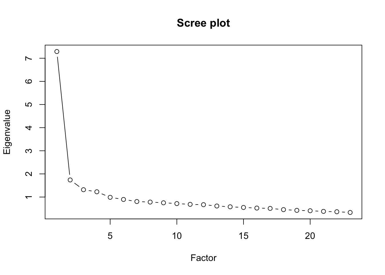
We see from the output that there are 4 factors - the Kaiser criterion shows 4 factors (eigenvalues \(>1\)) and the scree plot confirms this.
We now proceed with the factor analysis with 4 factors.
install.packages("GPArotation")library(GPArotation)
fa<-fa(q,nfactors = 4, rotate="none",fm="pa")
faFactor Analysis using method = pa
Call: fa(r = q, nfactors = 4, rotate = "none", fm = "pa")
Standardized loadings (pattern matrix) based upon correlation matrix
PA1 PA2 PA3 PA4 h2 u2 com
Question_01 0.56 0.11 -0.09 0.21 0.37 0.63 1.4
Question_02 -0.28 0.37 0.18 0.10 0.26 0.74 2.6
Question_03 -0.61 0.25 0.20 -0.05 0.47 0.53 1.6
Question_04 0.61 0.08 -0.05 0.20 0.42 0.58 1.3
Question_05 0.52 0.04 -0.01 0.16 0.30 0.70 1.2
Question_06 0.55 0.02 0.49 -0.22 0.59 0.41 2.3
Question_07 0.66 -0.02 0.22 0.01 0.49 0.51 1.2
Question_08 0.55 0.48 -0.28 -0.19 0.65 0.35 2.8
Question_09 -0.27 0.46 0.14 0.19 0.34 0.66 2.2
Question_10 0.40 -0.01 0.16 -0.09 0.20 0.80 1.4
Question_11 0.65 0.31 -0.22 -0.26 0.63 0.37 2.1
Question_12 0.64 -0.10 0.07 0.16 0.45 0.55 1.2
Question_13 0.65 0.02 0.21 -0.08 0.47 0.53 1.2
Question_14 0.63 -0.04 0.16 0.05 0.42 0.58 1.2
Question_15 0.56 -0.01 0.04 -0.09 0.32 0.68 1.1
Question_16 0.65 -0.02 -0.09 0.15 0.46 0.54 1.1
Question_17 0.63 0.36 -0.17 -0.14 0.58 0.42 1.9
Question_18 0.68 -0.04 0.27 0.01 0.54 0.46 1.3
Question_19 -0.40 0.27 0.12 0.05 0.24 0.76 2.0
Question_20 0.41 -0.15 -0.21 0.18 0.27 0.73 2.3
Question_21 0.63 -0.08 -0.08 0.23 0.47 0.53 1.3
Question_22 -0.28 0.29 0.07 0.28 0.25 0.75 3.1
Question_23 -0.13 0.18 0.10 0.24 0.12 0.88 2.9
PA1 PA2 PA3 PA4
SS loadings 6.74 1.13 0.81 0.62
Proportion Var 0.29 0.05 0.04 0.03
Cumulative Var 0.29 0.34 0.38 0.40
Proportion Explained 0.72 0.12 0.09 0.07
Cumulative Proportion 0.72 0.85 0.93 1.00
Mean item complexity = 1.8
Test of the hypothesis that 4 factors are sufficient.
df null model = 253 with the objective function = 7.55 with Chi Square = 19334.49
df of the model are 167 and the objective function was 0.46
The root mean square of the residuals (RMSR) is 0.03
The df corrected root mean square of the residuals is 0.03
The harmonic n.obs is 2571 with the empirical chi square 880.48 with prob < 2.3e-97
The total n.obs was 2571 with Likelihood Chi Square = 1166.49 with prob < 2.1e-149
Tucker Lewis Index of factoring reliability = 0.921
RMSEA index = 0.048 and the 90 % confidence intervals are 0.046 0.051
BIC = -144.8
Fit based upon off diagonal values = 0.99
Measures of factor score adequacy
PA1 PA2 PA3 PA4
Correlation of (regression) scores with factors 0.96 0.82 0.79 0.72
Multiple R square of scores with factors 0.93 0.68 0.63 0.52
Minimum correlation of possible factor scores 0.85 0.35 0.26 0.05- An inspection of the Pattern Matrix in the output shows that it is currently difficult to identify these factors (no clear distinction between high and low loadings). We therefore perform a rotation. We first employ an oblique Oblimin rotation.
fa2<-fa(q,nfactors = 4, rotate="oblimin",fm="pa")
fa2
Factor Analysis using method = pa
Call: fa(r = q, nfactors = 4, rotate = "oblimin", fm = "pa")
Standardized loadings (pattern matrix) based upon correlation matrix
PA1 PA3 PA4 PA2 h2 u2 com
Question_01 0.51 0.02 0.19 0.08 0.37 0.63 1.3
Question_02 -0.11 0.06 0.03 0.48 0.26 0.74 1.2
Question_03 -0.42 0.03 -0.09 0.36 0.47 0.53 2.1
Question_04 0.53 0.08 0.15 0.06 0.42 0.58 1.2
Question_05 0.43 0.11 0.10 0.03 0.30 0.70 1.3
Question_06 -0.11 0.81 0.02 0.00 0.59 0.41 1.0
Question_07 0.29 0.47 0.04 -0.03 0.49 0.51 1.7
Question_08 -0.01 -0.07 0.84 0.06 0.65 0.35 1.0
Question_09 0.00 -0.01 0.07 0.59 0.34 0.66 1.0
Question_10 0.05 0.35 0.08 -0.07 0.20 0.80 1.2
Question_11 -0.03 0.07 0.75 -0.11 0.63 0.37 1.1
Question_12 0.50 0.24 -0.03 -0.07 0.45 0.55 1.5
Question_13 0.16 0.49 0.13 -0.05 0.47 0.53 1.4
Question_14 0.33 0.38 0.03 -0.04 0.42 0.58 2.0
Question_15 0.15 0.27 0.20 -0.14 0.32 0.68 3.0
Question_16 0.51 0.07 0.15 -0.08 0.46 0.54 1.3
Question_17 0.10 0.07 0.67 0.03 0.58 0.42 1.1
Question_18 0.29 0.53 0.00 -0.03 0.54 0.46 1.6
Question_19 -0.19 -0.03 -0.02 0.36 0.24 0.76 1.6
Question_20 0.48 -0.15 0.02 -0.17 0.27 0.73 1.5
Question_21 0.61 0.05 0.03 -0.07 0.47 0.53 1.0
Question_22 0.15 -0.12 -0.08 0.48 0.25 0.75 1.4
Question_23 0.17 -0.02 -0.11 0.35 0.12 0.88 1.7
PA1 PA3 PA4 PA2
SS loadings 3.14 2.39 2.29 1.49
Proportion Var 0.14 0.10 0.10 0.06
Cumulative Var 0.14 0.24 0.34 0.40
Proportion Explained 0.34 0.26 0.25 0.16
Cumulative Proportion 0.34 0.59 0.84 1.00
With factor correlations of
PA1 PA3 PA4 PA2
PA1 1.00 0.51 0.54 -0.39
PA3 0.51 1.00 0.46 -0.30
PA4 0.54 0.46 1.00 -0.20
PA2 -0.39 -0.30 -0.20 1.00
Mean item complexity = 1.4
Test of the hypothesis that 4 factors are sufficient.
df null model = 253 with the objective function = 7.55 with Chi Square = 19334.49
df of the model are 167 and the objective function was 0.46
The root mean square of the residuals (RMSR) is 0.03
The df corrected root mean square of the residuals is 0.03
The harmonic n.obs is 2571 with the empirical chi square 880.48 with prob < 2.3e-97
The total n.obs was 2571 with Likelihood Chi Square = 1166.49 with prob < 2.1e-149
Tucker Lewis Index of factoring reliability = 0.921
RMSEA index = 0.048 and the 90 % confidence intervals are 0.046 0.051
BIC = -144.8
Fit based upon off diagonal values = 0.99
Measures of factor score adequacy
PA1 PA3 PA4 PA2
Correlation of (regression) scores with factors 0.91 0.90 0.92 0.82
Multiple R square of scores with factors 0.83 0.81 0.84 0.67
Minimum correlation of possible factor scores 0.66 0.62 0.69 0.35- Since not all of the \(|\text{factor correlations}|> 0.32\) we use a varimax rotation using:
fa3<-fa(q,nfactors = 4, rotate="varimax",fm="pa")
fa3- In order to make identifying the factors easier we hide loadings smaller than 0.3 using the following R code:
print(fa3$loadings, digits=2, cutoff=.3, sort=TRUE)
Loadings:
            PA1   PA3   PA4   PA2
Question_01  0.50
Question_03 -0.50              0.40
Question_04  0.53
Question_12  0.51  0.40
Question_16  0.54
Question_21  0.59
Question_06        0.75
Question_07  0.36  0.56
Question_13        0.56
Question_18  0.37  0.61
Question_08              0.76
Question_11              0.69
Question_17              0.64
Question_09                    0.56
Question_02                    0.46
Question_05  0.44
Question_10        0.38
Question_14  0.39  0.49
Question_15        0.38
Question_19                    0.38
Question_20  0.46
Question_22                    0.47
Question_23                    0.33

                PA1  PA3  PA4  PA2
SS loadings    3.03 2.85 1.99 1.44
Proportion Var 0.13 0.12 0.09 0.06
Cumulative Var 0.13 0.26 0.34 0.40- An inspection of the rotated pattern matrix now shows the factors more clearly. In particular, we see that:
- Factor 1 represents questions directly related to statistics (Questions 1,3,4,5,12,16,20,21);
- Factor 2 represents questions directly related to computing (Questions 6,7,10,13,14,15,18);
- Factor 3 represents questions directly related to mathematics (Questions 8,11,17);
- Factor 4 represents questions related to peer pressure (Questions 2, 9,19,22,23).
Exercise 1
Perform a factor analysis on the Factor Analysis (Scholarship Tests) dataset to determine the main underlying factors in the variables. It is important to note that the variables pairnum, sex and zygosity should not be included in your analysis as they are not in the correct form, i.e. they are not ordered categorical with 5 or more categories, nor are they continuous.
With respect to assumptions, linearity and no outliers may be assumed, however all other assumptions must be checked.
Hint: This dataset contains a number of ``NA” entries which cause a problem for the analyses. These can be removed using the following code (assuming the name allocated to the dataset when importing into R is Scholarship):
Scholarship2<-na.omit(Scholarship)
attach(Scholarship2)
head(Scholarship2)
Solution
library(foreign)
Scholarship<-read.spss(file.choose(), to.data.frame = T)- This dataset contains a number of “NA” terms. We need to remove these using the following command:
Scholarship2<-na.omit(Scholarship)
attach(Scholarship2)
head(Scholarship2)
pairnum sex zygosity moed faed faminc english math socsci natsci vocab
1 1 2 1 3 4 2 14 13 17 18 14
2 1 2 1 3 4 2 11 14 15 10 12
3 4 2 1 1 1 1 20 20 16 16 13
4 4 2 1 1 1 1 17 19 13 13 14
5 5 2 1 1 1 1 11 8 15 16 12
6 5 2 1 1 1 1 16 13 13 8 15- Here we create a list of variables that we wish to reduce.
q2<-cbind(moed,faed,faminc,english,math,socsci,natsci,vocab)- In order to check the no extreme multicollinearity assumption we calculate det(correlation matrix):
cor2<-cor(q2)
det(cor2)
[1] 0.02232106Clearly this is >0.00001, satisfying the assumption.
We next check the factorability using the KMO test and Bartlett’s test.
install.packages("psych")library(psych)
KMO(cor2)Kaiser-Meyer-Olkin factor adequacy
Call: KMO(r = cor2)
Overall MSA = 0.84
MSA for each item =
moed faed faminc english math socsci natsci vocab
0.74 0.73 0.80 0.91 0.89 0.84 0.86 0.84 cortest.bartlett(cor2)Warning in cortest.bartlett(cor2): n not specified, 100 used$chisq
[1] 363.1125
$p.value
[1] 5.702513e-60
$df
[1] 28Both of these tests indicate factorability.
In order to determine the number of factors we calculate and plot the eignevalues. We see that we have 2 factors.
eigen<-eigen(cor2)
val2<-eigen$values
val2
[1] 3.8819043 1.6423958 0.6028013 0.5428420 0.4138375 0.3904173 0.3167284
[8] 0.2090733plot(val2, type="b", ylab="Eigenvalue", xlab="Factor", main="Scree plot")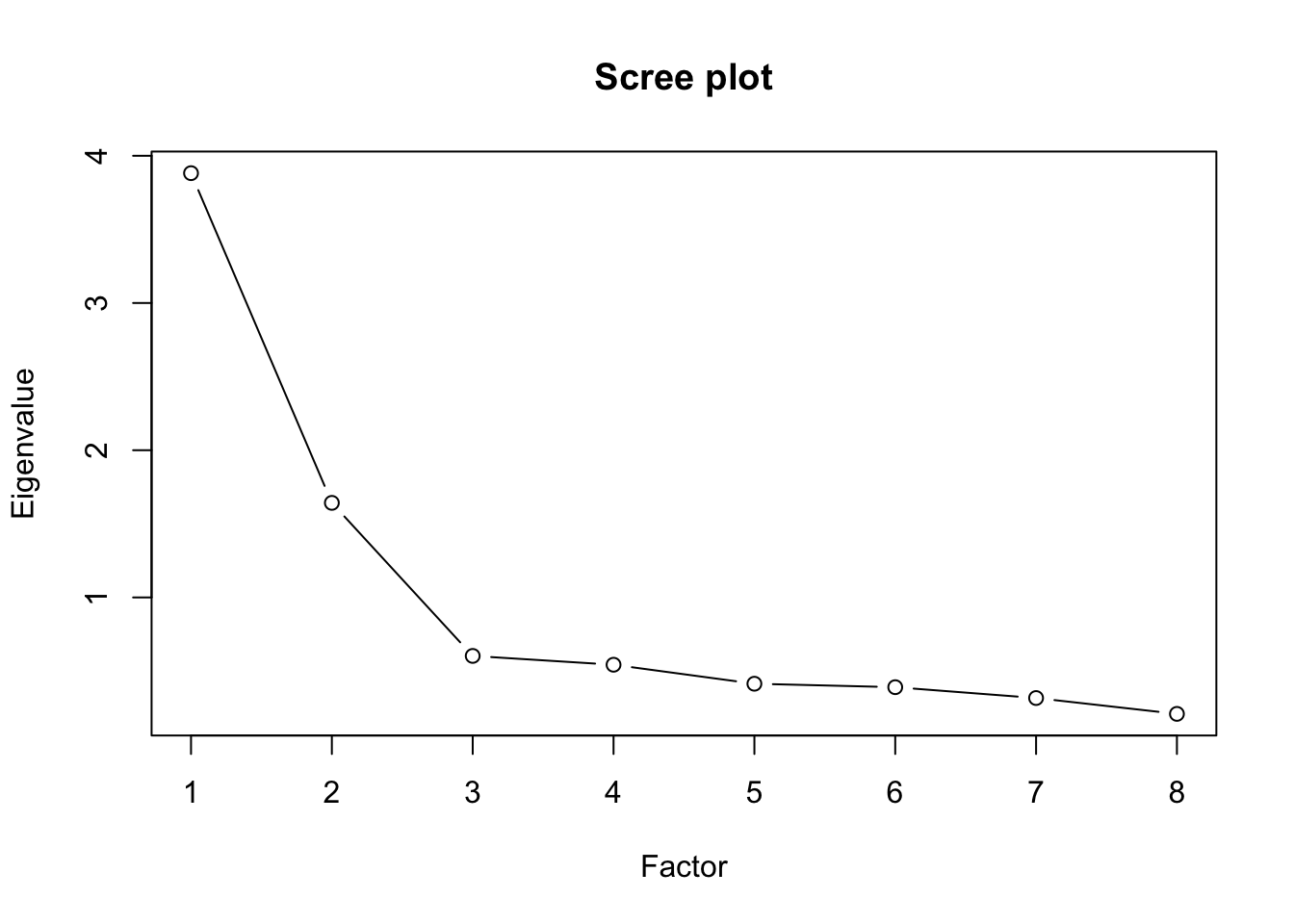
- We now proceed with the factor analysis with 2 factors
install.packages("GPArotation")library(GPArotation)
fa4<-fa(q2,nfactors = 2, rotate="none",fm="pa")
fa4Factor Analysis using method = pa
Call: fa(r = q2, nfactors = 2, rotate = "none", fm = "pa")
Standardized loadings (pattern matrix) based upon correlation matrix
PA1 PA2 h2 u2 com
moed 0.37 0.54 0.43 0.57 1.8
faed 0.49 0.69 0.72 0.28 1.8
faminc 0.39 0.48 0.38 0.62 1.9
english 0.73 -0.18 0.57 0.43 1.1
math 0.72 -0.12 0.54 0.46 1.1
socsci 0.84 -0.24 0.76 0.24 1.2
natsci 0.75 -0.24 0.62 0.38 1.2
vocab 0.82 -0.14 0.69 0.31 1.1
PA1 PA2
SS loadings 3.51 1.20
Proportion Var 0.44 0.15
Cumulative Var 0.44 0.59
Proportion Explained 0.75 0.25
Cumulative Proportion 0.75 1.00
Mean item complexity = 1.4
Test of the hypothesis that 2 factors are sufficient.
df null model = 28 with the objective function = 3.8 with Chi Square = 5823.11
df of the model are 13 and the objective function was 0.15
The root mean square of the residuals (RMSR) is 0.03
The df corrected root mean square of the residuals is 0.04
The harmonic n.obs is 1536 with the empirical chi square 63.56 with prob < 1.2e-08
The total n.obs was 1536 with Likelihood Chi Square = 228.5 with prob < 1.8e-41
Tucker Lewis Index of factoring reliability = 0.92
RMSEA index = 0.104 and the 90 % confidence intervals are 0.092 0.116
BIC = 133.12
Fit based upon off diagonal values = 1
Measures of factor score adequacy
PA1 PA2
Correlation of (regression) scores with factors 0.95 0.87
Multiple R square of scores with factors 0.91 0.76
Minimum correlation of possible factor scores 0.82 0.52- As it is not clear from the factor loadings what the factors represent, we perfom an rotation
fa5<-fa(q2,nfactors = 2, rotate="oblimin",fm="pa")
fa5
Factor Analysis using method = pa
Call: fa(r = q2, nfactors = 2, rotate = "oblimin", fm = "pa")
Standardized loadings (pattern matrix) based upon correlation matrix
PA1 PA2 h2 u2 com
moed -0.01 0.66 0.43 0.57 1
faed 0.00 0.85 0.72 0.28 1
faminc 0.04 0.60 0.38 0.62 1
english 0.75 0.00 0.57 0.43 1
math 0.71 0.06 0.54 0.46 1
socsci 0.88 -0.04 0.76 0.24 1
natsci 0.81 -0.05 0.62 0.38 1
vocab 0.81 0.07 0.69 0.31 1
PA1 PA2
SS loadings 3.16 1.54
Proportion Var 0.40 0.19
Cumulative Var 0.40 0.59
Proportion Explained 0.67 0.33
Cumulative Proportion 0.67 1.00
With factor correlations of
PA1 PA2
PA1 1.00 0.36
PA2 0.36 1.00
Mean item complexity = 1
Test of the hypothesis that 2 factors are sufficient.
df null model = 28 with the objective function = 3.8 with Chi Square = 5823.11
df of the model are 13 and the objective function was 0.15
The root mean square of the residuals (RMSR) is 0.03
The df corrected root mean square of the residuals is 0.04
The harmonic n.obs is 1536 with the empirical chi square 63.56 with prob < 1.2e-08
The total n.obs was 1536 with Likelihood Chi Square = 228.5 with prob < 1.8e-41
Tucker Lewis Index of factoring reliability = 0.92
RMSEA index = 0.104 and the 90 % confidence intervals are 0.092 0.116
BIC = 133.12
Fit based upon off diagonal values = 1
Measures of factor score adequacy
PA1 PA2
Correlation of (regression) scores with factors 0.95 0.90
Multiple R square of scores with factors 0.90 0.80
Minimum correlation of possible factor scores 0.81 0.61Since all of the |factor correlations|> 0.32, we stick to this rotation.
Factor 1 is associated with family factors, while Factor 2 is associated with subject tests.
Example 2
In this example we will use a principal component analysis (PCA) to try to reduce the number of variables in the Iris dataset into a smaller number of components. The dataset contains information on iris plants and clearly we ignore the species variable as it is not in the correct format for the procedure.
As in the factor analysis example, we will assume the assumptions of linearity (scatterplots may be used for this) and no outliers, but we will investigate the assumptions of no extreme multicollinearity and factorability. The data is ordered categorical and \(n=150\), which is sufficient. Follow the steps below:
- We use the in-built dataset Iris for this example. We invoke and check the dataset using the following code in R:
library(datasets)
head(iris)
Sepal.Length Sepal.Width Petal.Length Petal.Width Species
1 5.1 3.5 1.4 0.2 setosa
2 4.9 3.0 1.4 0.2 setosa
3 4.7 3.2 1.3 0.2 setosa
4 4.6 3.1 1.5 0.2 setosa
5 5.0 3.6 1.4 0.2 setosa
6 5.4 3.9 1.7 0.4 setosaattach(iris)- Next we create a list of variables that we wish to reduce.
x<-cbind(Sepal.Length,Sepal.Width, Petal.Length, Petal.Width)- In order to check the no extreme multicollinearity assumption we calculate det(correlation matrix):
cor3<-cor(x)
det(cor3)
[1] 0.008109611From the above output, we see that \(\det(\text{correlation matrix})=0.008>0.00001\) which satisfies the no extreme multicollinearity assumption.
We next check the factorability using the KMO test and Bartlett’s test.
library(psych)
KMO(cor3)
Kaiser-Meyer-Olkin factor adequacy
Call: KMO(r = cor3)
Overall MSA = 0.54
MSA for each item =
Sepal.Length Sepal.Width Petal.Length Petal.Width
0.58 0.27 0.53 0.63 cortest.bartlett(cor3)$chisq
[1] 466.224
$p.value
[1] 1.579704e-97
$df
[1] 6The KMO statistic is \(0.54>0.5\) and Bartlett’s test is significant, therefore satisfying the factorability assumption.
We next perform PCA with the in-built command.
pca <- prcomp(iris[c(1:4)], center = T, scale=T)
summary(pca)
Importance of components:
PC1 PC2 PC3 PC4
Standard deviation 1.7084 0.9560 0.38309 0.14393
Proportion of Variance 0.7296 0.2285 0.03669 0.00518
Cumulative Proportion 0.7296 0.9581 0.99482 1.00000- We also see from the output that the Kaiser criterion suggests only 1 component (the eigenvalues are given in the “Standard deviation” row). However, closer inspection of the scree plot shows a clear cut-off after two components. Use the code below to produce the scree plot:
plot(pca, type="l")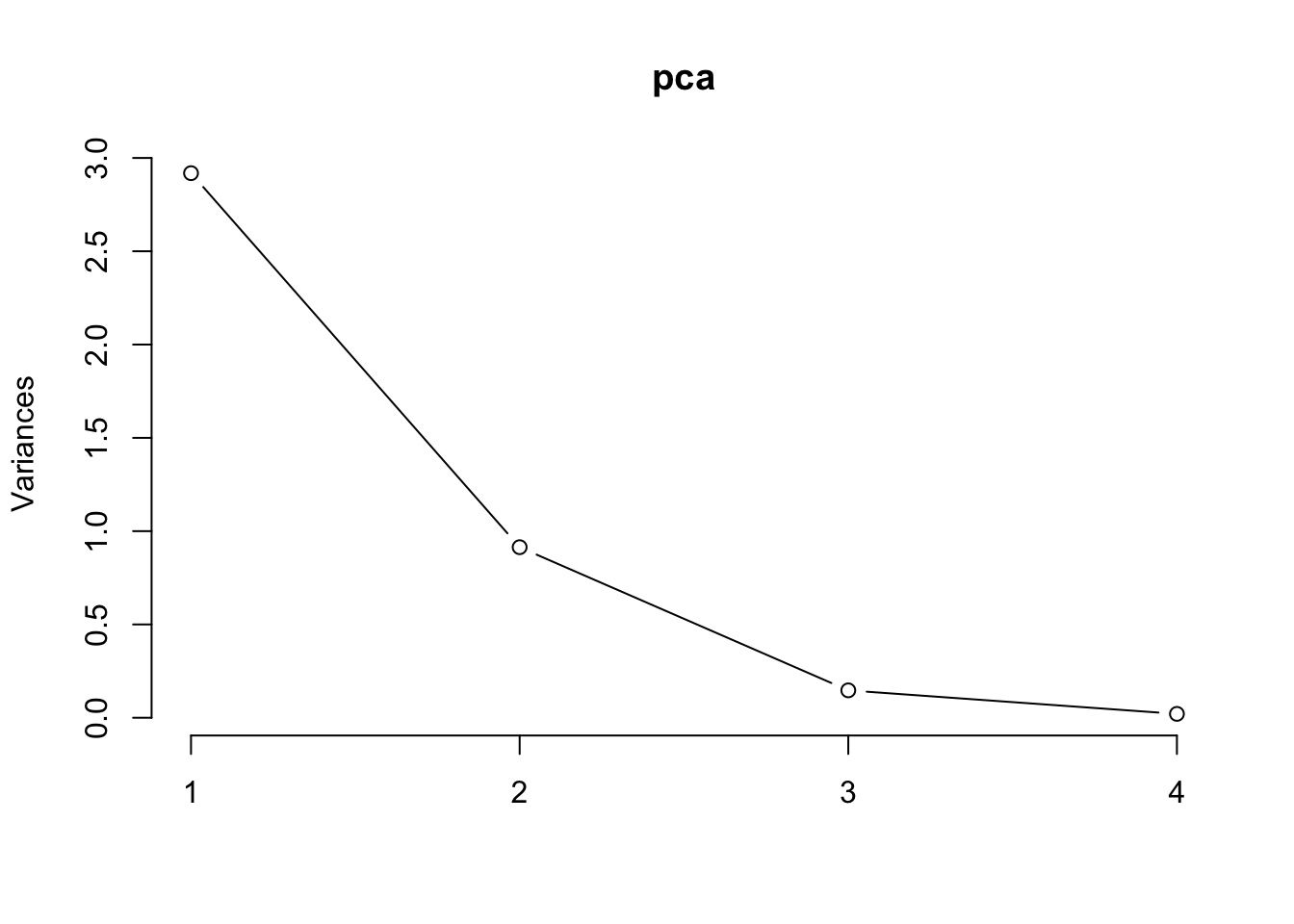
- Sometimes a biplot can help visualise the components:
biplot(pca, scale=0)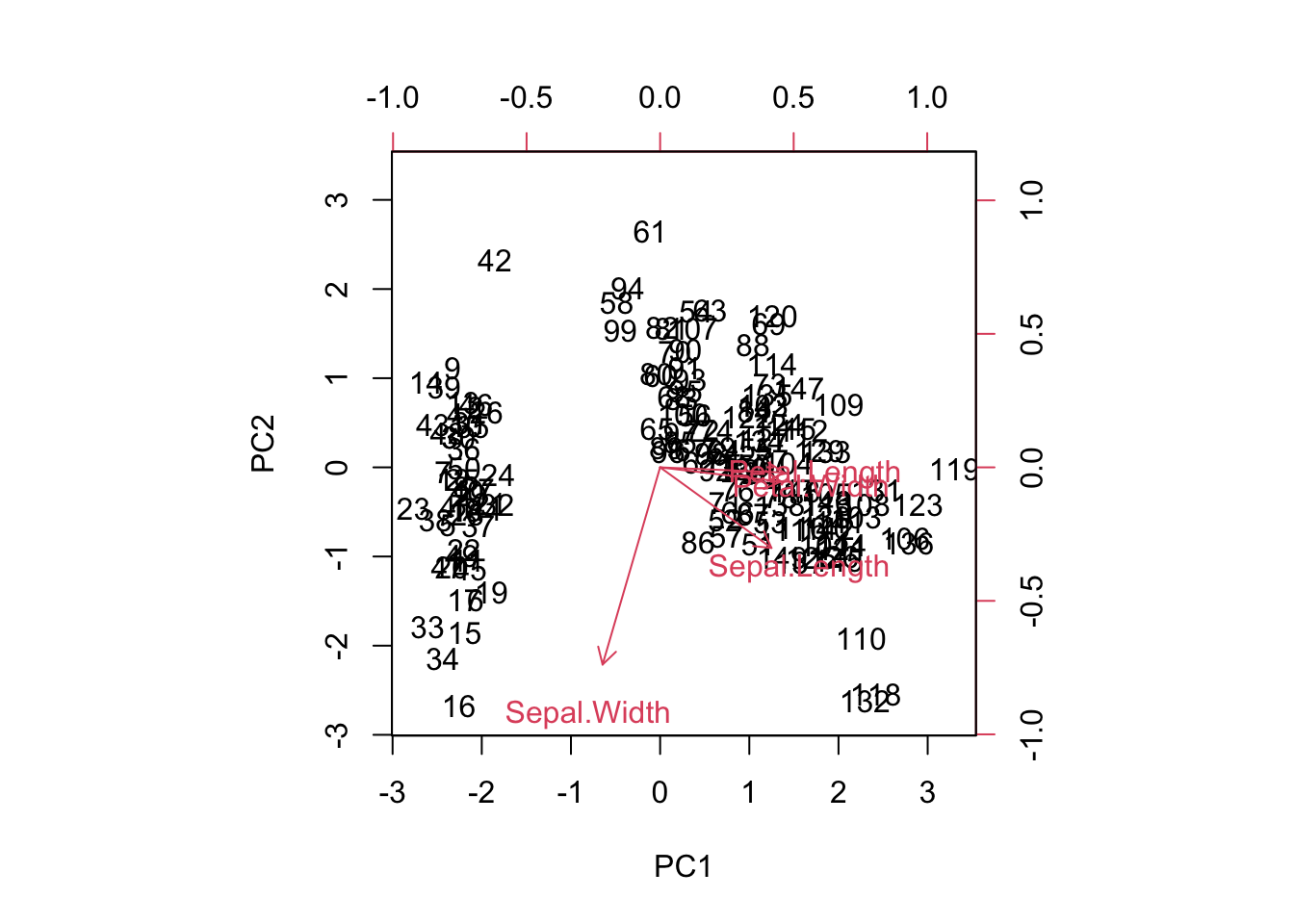
- We may also use the component loadings (using the 2 identified components) to identify the components:
library(psych)
pca2 <- principal(x,2,rotate="none")
pca2
Principal Components Analysis
Call: principal(r = x, nfactors = 2, rotate = "none")
Standardized loadings (pattern matrix) based upon correlation matrix
PC1 PC2 h2 u2 com
Sepal.Length 0.89 0.36 0.92 0.0774 1.3
Sepal.Width -0.46 0.88 0.99 0.0091 1.5
Petal.Length 0.99 0.02 0.98 0.0163 1.0
Petal.Width 0.96 0.06 0.94 0.0647 1.0
PC1 PC2
SS loadings 2.92 0.91
Proportion Var 0.73 0.23
Cumulative Var 0.73 0.96
Proportion Explained 0.76 0.24
Cumulative Proportion 0.76 1.00
Mean item complexity = 1.2
Test of the hypothesis that 2 components are sufficient.
The root mean square of the residuals (RMSR) is 0.03
with the empirical chi square 1.72 with prob < NA
Fit based upon off diagonal values = 1- As it is not clear from the component loadings what the components represent, we perform a rotation (oblique first)
library(GPArotation)
pca3 <- principal(x,2,rotate="oblimin")
pca3
Principal Components Analysis
Call: principal(r = x, nfactors = 2, rotate = "oblimin")
Standardized loadings (pattern matrix) based upon correlation matrix
TC1 TC2 h2 u2 com
Sepal.Length 1.00 0.20 0.92 0.0774 1.1
Sepal.Width -0.02 0.99 0.99 0.0091 1.0
Petal.Length 0.94 -0.16 0.98 0.0163 1.1
Petal.Width 0.93 -0.11 0.94 0.0647 1.0
TC1 TC2
SS loadings 2.75 1.08
Proportion Var 0.69 0.27
Cumulative Var 0.69 0.96
Proportion Explained 0.72 0.28
Cumulative Proportion 0.72 1.00
With component correlations of
TC1 TC2
TC1 1.00 -0.27
TC2 -0.27 1.00
Mean item complexity = 1
Test of the hypothesis that 2 components are sufficient.
The root mean square of the residuals (RMSR) is 0.03
with the empirical chi square 1.72 with prob < NA
Fit based upon off diagonal values = 1- Since not all of the \(|\text{component correlations}|> 0.32\) we use a varimax rotation:
pca4 <- principal(x,2,rotate="varimax")
pca4
Principal Components Analysis
Call: principal(r = x, nfactors = 2, rotate = "varimax")
Standardized loadings (pattern matrix) based upon correlation matrix
RC1 RC2 h2 u2 com
Sepal.Length 0.96 0.05 0.92 0.0774 1.0
Sepal.Width -0.14 0.98 0.99 0.0091 1.0
Petal.Length 0.94 -0.30 0.98 0.0163 1.2
Petal.Width 0.93 -0.26 0.94 0.0647 1.2
RC1 RC2
SS loadings 2.70 1.13
Proportion Var 0.68 0.28
Cumulative Var 0.68 0.96
Proportion Explained 0.71 0.29
Cumulative Proportion 0.71 1.00
Mean item complexity = 1.1
Test of the hypothesis that 2 components are sufficient.
The root mean square of the residuals (RMSR) is 0.03
with the empirical chi square 1.72 with prob < NA
Fit based upon off diagonal values = 1- Removing the smaller loadings with the following code makes identifying the components easier.
print(pca4$loadings, digits=2, cutoff=.4, sort=TRUE)
Loadings:
             RC1   RC2
Sepal.Length  0.96
Petal.Length  0.94
Petal.Width   0.93
Sepal.Width         0.98

                RC1  RC2
SS loadings    2.70 1.13
Proportion Var 0.68 0.28
Cumulative Var 0.68 0.96- Using this output, together with the biplot above, we see that one component is made up of sepal length, petal length and petal width, while the second component is sepal width only.
Exercise 2
Perform a principal component analysis on the Places dataset to determine the main underlying components in the variables. With respect to assumptions, linearity and no outliers may be assumed, however all other assumptions must be checked.
Solutions
Places<-read.csv(file.choose(), header = T)head(Places) Climate_and_Terrain Housing Health_Care_and_Environment Crime Transportation
1 521 6200 237 923 4031
2 575 8138 1656 886 4883
3 468 7339 618 970 2531
4 476 7908 1431 610 6883
5 659 8393 1853 1483 6558
6 520 5819 640 727 2444
Education The_Arts Recreation Economics
1 2757 996 1405 7633
2 2438 5564 2632 4350
3 2560 237 859 5250
4 3399 4655 1617 5864
5 3026 4496 2612 5727
6 2972 334 1018 5254attach(Places)- Here we create a list of variables that we wish to reduce.
x2<-cbind(Climate_and_Terrain, Housing, Health_Care_and_Environment, Crime, Transportation,
Education, The_Arts, Recreation, Economics)- In order to check the no extreme multicollinearity assumption we calculate det(correlation matrix):
cor4<-cor(x2)
det(cor4)
[1] 0.03900546Clearly this is >0.00001, satisfying the assumption.
We next check the factorability using the KMO test and Bartlett’s test.
library(psych)
KMO(cor4)
Kaiser-Meyer-Olkin factor adequacy
Call: KMO(r = cor4)
Overall MSA = 0.7
MSA for each item =
Climate_and_Terrain Housing
0.55 0.69
Health_Care_and_Environment Crime
0.69 0.64
Transportation Education
0.86 0.74
The_Arts Recreation
0.71 0.81
Economics
0.38 cortest.bartlett(cor4)$chisq
[1] 308.7258
$p.value
[1] 4.629125e-45
$df
[1] 36Both of these tests indicate factorability.
We next perform PCA with the in-built command.
pca5 <- prcomp(x2, center = T, scale=T)
summary(pca5)
Importance of components:
PC1 PC2 PC3 PC4 PC5 PC6 PC7
Standard deviation 1.8462 1.1018 1.0684 0.9596 0.8679 0.79408 0.70217
Proportion of Variance 0.3787 0.1349 0.1268 0.1023 0.0837 0.07006 0.05478
Cumulative Proportion 0.3787 0.5136 0.6404 0.7427 0.8264 0.89650 0.95128
PC8 PC9
Standard deviation 0.56395 0.34699
Proportion of Variance 0.03534 0.01338
Cumulative Proportion 0.98662 1.00000*We now produce a scree plot
plot(pca5, type="l")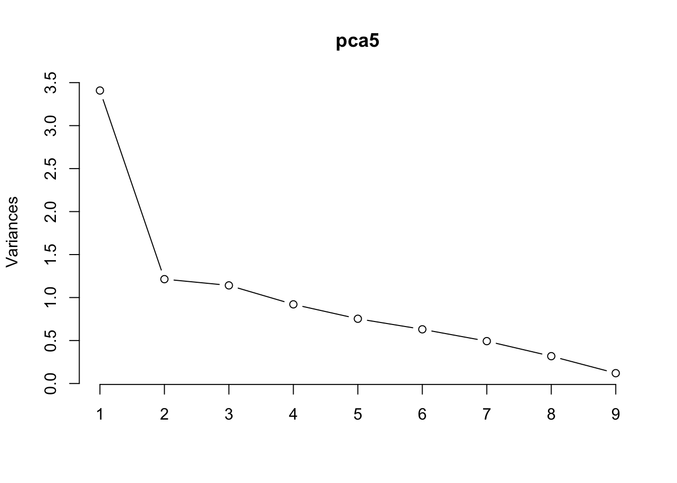
The evidence suggest that we use 3 components.
A biplot is sometimes useful in identifying the components, but we see in this case that is of less use due to its complicated nature.
biplot(pca5, scale=0)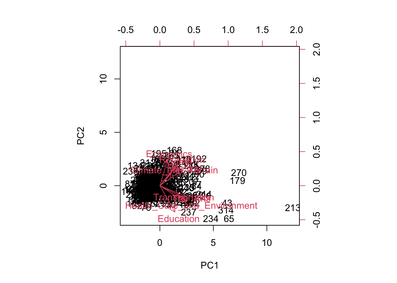
- We may also use the component loadings (using the 3 identified components) to identify the components:
library(GPArotation)
library(psych)
pca6 <- principal(x2,3,rotate="none")
pca6
Principal Components Analysis
Call: principal(r = x2, nfactors = 3, rotate = "none")
Standardized loadings (pattern matrix) based upon correlation matrix
PC1 PC2 PC3 h2 u2 com
Climate_and_Terrain 0.38 0.24 -0.74 0.75 0.25 1.7
Housing 0.66 0.28 -0.22 0.56 0.44 1.6
Health_Care_and_Environment 0.85 -0.33 -0.01 0.83 0.17 1.3
Crime 0.52 0.39 0.20 0.46 0.54 2.2
Transportation 0.65 -0.20 0.16 0.48 0.52 1.3
Education 0.51 -0.53 0.25 0.60 0.40 2.4
The_Arts 0.85 -0.21 -0.03 0.78 0.22 1.1
Recreation 0.61 0.42 -0.05 0.55 0.45 1.8
Economics 0.25 0.52 0.65 0.75 0.25 2.2
PC1 PC2 PC3
SS loadings 3.41 1.21 1.14
Proportion Var 0.38 0.13 0.13
Cumulative Var 0.38 0.51 0.64
Proportion Explained 0.59 0.21 0.20
Cumulative Proportion 0.59 0.80 1.00
Mean item complexity = 1.7
Test of the hypothesis that 3 components are sufficient.
The root mean square of the residuals (RMSR) is 0.11
with the empirical chi square 281.76 with prob < 3.1e-53
Fit based upon off diagonal values = 0.89- As it is not clear from the component loadings what the components represent, we perform a rotation (oblique first)
pca7 <- principal(x2,3,rotate="oblimin")
pca7
Principal Components Analysis
Call: principal(r = x2, nfactors = 3, rotate = "oblimin")
Standardized loadings (pattern matrix) based upon correlation matrix
TC1 TC3 TC2 h2 u2 com
Climate_and_Terrain -0.02 0.86 -0.18 0.75 0.25 1.1
Housing 0.26 0.55 0.25 0.56 0.44 1.9
Health_Care_and_Environment 0.88 0.11 -0.02 0.83 0.17 1.0
Crime 0.15 0.22 0.56 0.46 0.54 1.4
Transportation 0.66 -0.02 0.13 0.48 0.52 1.1
Education 0.81 -0.32 -0.11 0.60 0.40 1.3
The_Arts 0.80 0.19 0.06 0.78 0.22 1.1
Recreation 0.15 0.47 0.45 0.55 0.45 2.2
Economics -0.06 -0.18 0.87 0.75 0.25 1.1
TC1 TC3 TC2
SS loadings 2.72 1.57 1.47
Proportion Var 0.30 0.17 0.16
Cumulative Var 0.30 0.48 0.64
Proportion Explained 0.47 0.27 0.25
Cumulative Proportion 0.47 0.75 1.00
With component correlations of
TC1 TC3 TC2
TC1 1.00 0.27 0.21
TC3 0.27 1.00 0.08
TC2 0.21 0.08 1.00
Mean item complexity = 1.4
Test of the hypothesis that 3 components are sufficient.
The root mean square of the residuals (RMSR) is 0.11
with the empirical chi square 281.76 with prob < 3.1e-53
Fit based upon off diagonal values = 0.89- Since not all the the |component correlations|> 0.32, we use a varimax rotation:
pca8 <- principal(x2,3,rotate="varimax")
pca8
Principal Components Analysis
Call: principal(r = x2, nfactors = 3, rotate = "varimax")
Standardized loadings (pattern matrix) based upon correlation matrix
RC1 RC3 RC2 h2 u2 com
Climate_and_Terrain 0.01 0.85 -0.13 0.75 0.25 1.0
Housing 0.30 0.61 0.31 0.56 0.44 2.0
Health_Care_and_Environment 0.86 0.30 0.10 0.83 0.17 1.3
Crime 0.20 0.26 0.59 0.46 0.54 1.6
Transportation 0.65 0.12 0.21 0.48 0.52 1.3
Education 0.76 -0.15 -0.02 0.60 0.40 1.1
The_Arts 0.79 0.36 0.17 0.78 0.22 1.5
Recreation 0.20 0.51 0.50 0.55 0.45 2.3
Economics 0.00 -0.17 0.85 0.75 0.25 1.1
RC1 RC3 RC2
SS loadings 2.53 1.71 1.52
Proportion Var 0.28 0.19 0.17
Cumulative Var 0.28 0.47 0.64
Proportion Explained 0.44 0.30 0.26
Cumulative Proportion 0.44 0.74 1.00
Mean item complexity = 1.5
Test of the hypothesis that 3 components are sufficient.
The root mean square of the residuals (RMSR) is 0.11
with the empirical chi square 281.76 with prob < 3.1e-53
Fit based upon off diagonal values = 0.89- Removing the smaller loadings with the following code makes identifying the components easier.
print(pca8$loadings, digits=2, cutoff=.4, sort=TRUE)
Loadings:
                            RC1   RC3   RC2
Health_Care_and_Environment  0.86
Transportation               0.65
Education                    0.76
The_Arts                     0.79
Climate_and_Terrain                0.85
Housing                            0.61
Recreation                         0.51  0.50
Crime                                    0.59
Economics                                0.85

                RC1  RC3  RC2
SS loadings    2.53 1.71 1.52
Proportion Var 0.28 0.19 0.17
Cumulative Var 0.28 0.47 0.64- Using the rotated component matrix, we see that Health Care and Environment, Transportation, Education and The Arts form the first principal component. Intuitively, it makes sense that ratings for these are related. Climate and Terrain, Housing and Recreation form the second and Crime and Economics form the third principal component.